Sunday, December 20, 2015

HIVE

Understanding HIVE

Hive is a data warehousing infrastructure based on Hadoop. Hadoop provides massive scale out and fault tolerance capabilities for data storage and processing (using the map-reduce programming paradigm) on commodity hardware. Hive is designed to enable easy data summarization, ad-hoc querying and analysis of large volumes of data. It provides a simple query language called Hive QL, which is based on SQL and which enables users familiar with SQL to do ad-hoc querying, summarization and data analysis easily.
It is also to be noted that
  • Hive is not designed for online transaction processing and does not offer real-time queries and row level updates. It is best used for batch jobs over large sets of immutable data (like web logs).
  • Hive is not designed for online transaction processing and does not offer real-time queries and row level updates. It is best used for batch jobs over large sets of immutable data (like web logs).
Getting Started:
We will be using the same data that we used in our hive tutorial. Namely, files batting.csvand master.csv.

Data Source:


Accessing Hue
You can access HUE from the entering the address 127.0.0.1:8000
Login Id : Hue
Pwd : 1111
Uploading Data
Data is uploaded into the directory user/hue from the HDFS file system. The steps to upload the files into this directory are available on my previous blogs.
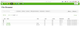
Once the files are uploaded they should look like this

Step 1 –  Load input file:

We need to unzip it into a directory.We will be uploading files from the data-set in “file browser” like below


In Hue there is a button called “Hive” and inside Hive there are query options like “Query Editor”, “My Queries” and “Tables” etc.
On left there is a “query editor”. A query may span multiple lines, there are buttons to Execute the query, Explain the query, Save the query with a name and to open a new window for another query.
Step 2 – Create empty table and load data in Hive
In “Table” we need to select “Create a new table from a file”, which will lead us to the “file browser”, where we will select “batting.csv” file and we will name the new table as “temp_batting


Data has been loaded, the file (batting.csv) will be deleted by HIVE.


We execute the following command, and this will show us the first 100 rows from
the table.


Step 3 – Creating a batting table and transfer data from the temporary table to batting table


Step 4 – Create a query to show the highest score per year
We will create a query to show the highest score per year by using “group by”.
 SELECT year, max(runs) FROM batting GROUP BY year;


Step 5- Get final result
We will execute final query which will show the player who scored the maximum runs in a year.


Hope this tutorial helps you in running the Hive Query Language for calculating baseball scores.

Thank you !!!


Friday, December 18, 2015

Workings on APACHE PIG in HADOOP

Previously we have seen how to write our first hadoop program now lets execute out first PIG program in hadoop


Learning PIG.....

Apache Pig is an open-source technology that offers a high-level mechanism for the parallel programming of MapReduce jobs to be executed on hadoop clusters

Pig enables developers to create query execution routines for analyzing large, distributed data sets without having to do low-level work in MapReduce, much like the way the ApacheHive data warehouse software provides a SQL-like interface for Hadoop that doesn't require direct MapReduce programming,
The key parts of Pig are a compiler and a scripting language known as Pig Latin. Pig Latin is a data-flow language geared toward parallel processing. Managers of the Apache software foundation's Pig project position the language as being part way between declarative SQL and the procedural JAVA approach used in MapReduce applications. Proponents say, for example, that data joins are easier to create with Pig Latin than with Java. However, through the use of user-defined functions (UDFs), Pig Latin applications can be extended to include custom processing tasks written in Java as well as languages such as JAVASCRIPT and Python.
Apache Pig grew out of work at Yahoo Research and was first formally described in a paper published in 2008. Pig is intended to handle all kinds of data, including structured and unstructured information and relational and nested data. That omnivorous view of data likely had a hand in the decision to name the environment for the common barnyard animal. It also extends to Pig's take on application frameworks; while the technology is primarily associated with Hadoop, it is said to be capable of being used with other frameworks as well.


Objective : 
We are going to read in a baseball statistics file. We are going to compute the highest runs by a player for each year. This file has all the statistics from 1871–2011 and it contains over 90,000 rows. Once we have the highest runs we will extend the script to translate a player id field into the first and last names of the players.

For free flow and continue along with the blog data can be downloaded from the following link.
http://hortonassets.s3.amazonaws.com/pig/lahman591-csv.zip

Like our previous blog run the hortonworks from the virtual box and after running it open the following link to do APACHE PIG , URL:http://127.0.0.1:8000

Login Details : 
Login : hue
password : 1111
You get to the hue screen as shown below and go to the file browser.


Once you have opened hue screen, navigate to file browser and upload the two csv files.


Once the files are uploaded click on the PIG icon on the top left corner of your screen to go to the PIG script page.

We need to write the following code and save it.

batting = load 'Batting.csv' using
PigStorage(',');
raw_runs = FILTER batting BY $1>0;
runs = FOREACH raw_runs GENERATE $0 as playerID, $1 as year, $8 as runs;
grp_data = GROUP runs by (year);
max_runs = FOREACH grp_data GENERATE group as grp,MAX(runs.runs) as max_runs;
join_max_run = JOIN max_runs by ($0, max_runs), runs by (year,runs);
join_data = FOREACH join_max_run GENERATE $0 as year, $2 as playerID, $1 as runs;
DUMP join_data;The explanation of above code is as follows:-
  1. We load data using a comma delimiter.
  2. Then we filter the first row of data.
  3. Iteration for batting data object.
  4. We should group the runs of each player by the year field.
  5. We then join the runs data of highest scoring player to obtain player ID.


Once the script is ready you hit the Execute button to start the job and it will show the job running status


Job Status
To  access this page you can either go to the job id which is displayed in bottom of the page when it says that the job is running successfully or go to Query History on the top left besides my scripts.


Once it is success you will get the following screen


Output will be obtained like below


Conclusion & Learning:
By this we have completed our task of executing the Pig script and obtaining the result of which player has highest runs from the year 1871 to 2011.

Excecuting First Program in HADOOP

 HADOOP

Hadoop is an open-source software framework for storing data and running applications on clusters of commodity hardware. It provides massive storage for any kind of data, enormous processing power and the ability to handle virtually limitless concurrent tasks or jobs.

BENEFITS OF HADOOP

Computing power. Its distributed computing model quickly processes big data. The more computing nodes you use, the more processing power you have.
Flexibility. Unlike traditional relational databases, you don’t have to preprocess data before storing it. You can store as much data as you want and decide how to use it later. That includes unstructured data like text, images and videos.
Fault tolerance. Data and application processing are protected against hardware failure. If a node goes down, jobs are automatically redirected to other nodes to make sure the distributed computing does not fail. And it automatically stores multiple copies of all data.
Low cost. The open-source framework is free and uses commodity hardware to store large quantities of data.

Scalability. You can easily grow your system simply by adding more nodes. Little administration is required

COMPONENTS COMPRISING HADOOP

Currently, four core modules are included in the basic framework from the Apache Foundation:
Hadoop Common – the libraries and utilities used by other Hadoop modules.
Hadoop Distributed File System (HDFS) – the Java-based scalable system that stores data across multiple machines without prior organization.
MapReduce – a software programming model for processing large sets of data in parallel.
YARN – resource management framework for scheduling and handling resource requests from distributed applications. (YARN is an acronym for Yet Another Resource Negotiator.)
Other software components that can run on top of or alongside Hadoop and have achieved top-level Apache project status include:

Pig – a platform for manipulating data stored in HDFS that includes a compiler for MapReduce programs and a high-level language called Pig Latin. It provides a way to perform data extractions, transformations and loading, and basic analysis without having to write MapReduce programs.
Hive – a data warehousing and SQL-like query language that presents data in the form of tables. Hive programming is similar to database programming. (It was initially developed by Facebook.)
HBase – a nonrelational, distributed database that runs on top of Hadoop. HBase tables can serve as input and output for MapReduce jobs.
HCatalog – a table and storage management layer that helps users share and access data.
Ambari – a web interface for managing, configuring and testing Hadoop services and components.
Cassandra – A distributed database system.
Chukwa – a data collection system for monitoring large distributed systems.
Flume – software that collects, aggregates and moves large amounts of streaming data into HDFS.
Oozie – a Hadoop job scheduler.
Sqoop – a connection and transfer mechanism that moves data between Hadoop and relational databases.
Spark – an open-source cluster computing framework with in-memory analytics.
Solr – an scalable search tool that includes indexing, reliability, central configuration, failover and recovery.
Zookeeper – an application that coordinates distributed processes.

In addition, there are commercial distributions of Hadoop, including Cloudera, Hortonworks and MapR. With distributions from software vendors, you pay for their version of the framework and receive additional software components, tools, training, documentation and other services.


EXECUTING THE FIRST PROGRAM IN HADOOP

Objective: 
We have to execute java coded MapReduce task of three large text files and count the frequency of words appeared in those text files using Hadoop under Hortonworks Data Platform installed on Oracle virtual box.

Framework: 

First install the  Oracle virtual box and then install hadoop in the virtual box and the installation will take some time.In the mean time have a COFFEE BREAK!!!!
After the installation whenever  you want to do something using hortonworks hadoop you need to click on start button in the virtual box which will take some time and give you the screen as below after the completion of installation


After installation process and obtaining the screen as above your system will become very slow don't panic because hadoop requires so much of RAM so I request you to have atleast 6-8 GB of RAM to run hadoop,if you cannot afford buying a system but hungry to learn BIG DATA check out the AWS service which comes with a certain trail period

Copy paste that URL in your web Browser which opens a window and go to the advanced settings and start the hortonworks
It will ask for a username and password
username: root
password: hadoop(but while typing password you will not see the cursor moving don't worry just type hadoop and press enter)
As we have java codes ready we need to create these java files using linux vi command. After editing the document we need to give the following commands to save and exit the editor shell. :w for writing and :q to quit from editor window and come back to shell box.
Please look at the editor window opened in my shell using 127.0.0.1:4200


 Below screen is where I edited my SumReducer.java, WordMapper.java and WordCount.java files.


Once your java files are ready for execution we need to create one new folder to save our class files which we are going to compile from java codes.
After creating a folder for class files. We have to execute the following code from shell.

javac -classpath /usr/hdp/2.3.0.0-2557/hadoop/hadoop-common-2.7.1.2.3.0.0-2557.jar:/usr/hdp/2.3.0.0-2557/hadoop-mapreduce/hadoop-mapreduce-client-core-2.7.1.2.3.0.0-2557.jar:/usr/hdp/2.3.0.0-2557/hadoop-mapreduce/commons-cli-1.2.jar -d WC-classes WordMapper.java
#-----
javac -classpath /usr/hdp/2.3.0.0-2557/hadoop/hadoop-common-2.7.1.2.3.0.0-2557.jar:/usr/hdp/2.3.0.0-2557/hadoop-mapreduce/hadoop-mapreduce-client-core-2.7.1.2.3.0.0-2557.jar:/usr/hdp/2.3.0.0-2557/hadoop-mapreduce/commons-cli-1.2.jar -d WC-classes SumReducer.java
#-----
javac -classpath /usr/hdp/2.3.0.0-2557/hadoop/hadoop-common-2.7.1.2.3.0.0-2557.jar:/usr/hdp/2.3.0.0-2557/hadoop-mapreduce/hadoop-mapreduce-client-core-2.7.1.2.3.0.0-2557.jar:/usr/hdp/2.3.0.0-2557/hadoop-mapreduce/commons-cli-1.2.jar:WCclasses -d WC-classes WordCount.java
#----

By using the code above we will be able to create class files of SumReducer, WordMapper & WordCount
What these programs essentially does is : we are having three large text files with lot of words. We are going to reduce this humongous task using reducer and mapper program

As we now have class files of SumReducer, WordMapper and WordCount we should create jar file using the following code.
<code> jar -cvf WordCount.jar -C WCclasses/ .</code>

Next step is to create folder in hdfs file system using the following commands.

<code>hdfs -mkdir user/ru1/wc-input</code>

After creating this folder we have to upload files using hue file browser using 127.0.0.1:8000 in our web browser.
After uploading files through file browser. It looks as follows.


Now its time to execute hadoop jar file. Let’s use the following code for doing the same.
hadoop jar WordCount.jar WordCount /user/ru1/wc-input /user/ru1/wc-out


After it is executed without any errors we need track the status of application in the all applications page using 127.0.0.1:8088
The screen looks as follows


 In this step we should see succeeded in the respective application. After confirming the success status we should open hue file browser where we will see a new folder created called wc-out2 (which we have given in shell command prompt).


 In this folder there will be two files called success and part-r-0000. The part-r-0000 is where we can check the output of the program and how many words are there and what is the frequency of each word occurred.


Thank You !


Friday, October 2, 2015

SAS - ASSIGNMENT-2 -SOLVED !

As a part of our ongoing Sas Curriculum, we are currently going through the book “Learning SAS® by Example “A Programmer’s Guide”” by Ron Cody.
  Below are the codes and explanations to practice problems from chapter 16-20, that we were given as a learning assignment , For each practice problem the codes and explanations are summarized as under–

The permanent library used for creating the data set and proc reports is A15007.
------libname a15007 "C:\Users\user\Desktop\sasbook\sas_assignment";

Chapter-16

Problem 1 and 2

1. Using the SAS data set College, compute the mean, median, minimum, and
maximum and the number of both missing and non-missing values for the variables
ClassRank and GPA. Report the statistics to two decimal places.
2. Repeat Problem 1, except compute the desired statistics for each combination of
Gender SchoolSize. Do this twice, once using a BY statement, and once using a
CLASS statement.

Code:

*Data set COLLEGE;
proc format library=a15007;
   value $yesno 'Y','1' = 'Yes'
                'N','0' = 'No'
                ' '     = 'Not Given';
   value $size 'S' = 'Small'
               'M' = 'Medium'
               'L' = 'Large'
                ' ' = 'Missing';
   value $gender 'F' = 'Female'
                 'M' = 'Male'
                 ' ' = 'Not Given';
run;
data a15007.college;
   length StudentID $ 5 Gender SchoolSize $ 1;
   do i = 1 to 100;
      StudentID = put(round(ranuni(123456)*10000),z5.);
      if ranuni(0) lt .4 then Gender = 'M';
      else Gender = 'F';
      if ranuni(0) lt .3 then SchoolSize = 'S';
      else if ranuni(0) lt .7 then SchoolSize = 'M';
      else SchoolSize = 'L';
      if ranuni(0) lt .2 then Scholarship = 'Y';
      else Scholarship = 'N';
      GPA = round(rannor(0)*.5 + 3.5,.01);
      if GPA gt 4 then GPA = 4;
      ClassRank = int(ranuni(0)*60 + 41);
      if ranuni(0) lt .1 then call missing(ClassRank);
      if ranuni(0) lt .05 then call missing(SchoolSize);
      if ranuni(0) lt .05 then call missing(GPA);
      output;
   end;
   format Gender $gender1. 
          SchoolSize $size. 
          Scholarship $yesno.;
   drop i;
run;

Problem- 1
options fmtsearch=(a15007); 
title "Statistics on the College Data Set";
proc means data=a15007.college
 n
 nmiss
 mean
 median
 min
 max
 maxdec=2;
 var ClassRank GPA;
run; 
proc sort data=a15007.college out=college;
 by Gender SchoolSize;
run; 

Problem - 2
title "Statistics on the College Data Set - Using BY";
title2 "Broken down by Gender and School Size";
proc means data=college
 n
 nmiss
 mean
 median
 min
 max
 maxdec=2;
 by Gender SchoolSize;
 var ClassRank GPA;
run; 

Output:


Problem 4

Repeat Problem 3 (CLASS statement only), except group small and medium school
sizes together. Do this by writing a new format for SchoolSize (values are S, M, and
L). Do not use any DATA steps.

Code

proc format;
 value $groupsize
 'S','M' = 'Small and Medium'
 'L' = 'Large';
run;

title "Statistics on the College Data Set";
title2 "Broken down by School Size";
proc means data=college
 n
 mean
 median
 min
 max
 maxdec=2;
 class SchoolSize;
 var ClassRank GPA;
 format SchoolSize $groupsize.; 
run; 

Output

Chapter - 17

Problem 2

Using the SAS data set BloodPressure, generate frequencies for the variable Age.
Use a user-defined format to group ages into three categories: 40 and younger, 41 to
60, and 61 and older. Use the appropriate options to omit the cumulative statistics
and percentages.

Code

/*Create Blood pressue data set*/
data a15007.bloodpressure;
   input Gender : $1. 
         Age
         SBP
         DBP;
datalines;
M 23 144 90
F 68 110 62
M 55 130 80
F 28 120 70
M 35 142 82
M 45 150 96
F 48 138 88
F 78 132 76
;

proc format;
 value agegrp low-40 = '40 and lower'
 41-60 = '41 to 60'
 61-high = '61 and higher';
run;
title "Using a Format to Regroup Values";
proc freq data=a15007.bloodpressure;
 tables age / nocum nopercent;
 format age agegrp.;
run; 

Output

Problem - 6

Using the SAS data set College, produce a three-way table of Gender (page) by
Scholarship (row) by SchoolSize (column).

Code

title "Three-way Tables";
proc freq data=a15007.college;
 tables Gender*Scholarship*SchoolSize;
run; 

Output


Chapter 18

Problem - 2

Produce the following table. Note that the ALL column has been renamed Total.
Demographics from COLLEGE Data Set


Code

title "Demographics from COLLEGE Data Set";
proc tabulate data=a15007.college format=6.;
 class Gender Scholarship SchoolSize;
 tables SchoolSize all,
 Gender Scholarship all/ rts=15;
 keylabel n=' '
 all = 'Total';
run; 

Output


Problem - 4

Produce the following table. Note that the keyword ALL has been renamed Total,
Gender is formatted, and ClassRank (a continuous numeric variable) has been
formatted into two groups (0–70 and 71 and higher).Demographics from COLLEGE Data Set

Code

proc format;
 value $gender 'F' = 'Female'
 'M' = 'Male';
 value rank low-70 = 'Low to 70'
 71-high = '71 and higher';
run;
title "Demographics from COLLEGE Data Set";
proc tabulate data=a15007.college format=6.;
 class Gender Scholarship ClassRank;
 tables Scholarship all,
 (ClassRank)*(Gender all) / rts=15;
 keylabel n=' '
 all = 'Total';
 format Gender $gender. ClassRank rank.;
run; 

Output


Chapter-19

Problem - 2

Run the same two procedures shown in Problem 1, except create a contents file, a
body file, and a frame file.

Code

ods listing close;
ods html body = 'prob19_2_body.html'
 contents = 'prob19_2_contents.html'
 frame = 'prob19_2_frame.html';

title "Using ODS to Create a Table of Contents";
proc print data=a15007.college(obs=8) noobs;
run;
proc means data=a15007.college n mean maxdec=2;
 var GPA ClassRank;
run;
ods html close;
ods listing; 

Output


Problem- 4

Send the results of a PROC PRINT on the data set Survey to an RTF file.

Code

*Data set SURVEY;
data a15007.survey;
   infile 'C:\Users\user\Desktop\sasbook\sas_assignment\survey.txt' pad;
   input ID : $3.
         Gender : $1.
         Age
         Salary
         (Ques1-Ques5)(1.);
run;
ods listing close;
ods rtf file='C:\Users\user\Desktop\sasbook\sas_assignment\prob19_4.rtf';
title "Demonstrating RTF Output";
proc print data=a15007.survey noobs;
run; 
ods rtf close;
ods listing; 

Output


Chapter-20

Problem-2

Repeat Problem 1, except produce a pie chart instead of a bar chart.

Code

*Data set BICYCLES;
data a15007.bicycles;
   input Country  & $25.
         Model    & $14.
         Manuf    : $10.
         Units    :   5.
         UnitCost :  comma8.;
   TotalSales = (Units * UnitCost) / 1000;
   format UnitCost TotalSales dollar10.;
   label TotalSales = "Sales in Thousands"
         Manuf = "Manufacturer";
datalines;
USA  Road Bike  Trek 5000 $2,200
USA  Road Bike  Cannondale 2000 $2,100
USA  Mountain Bike  Trek 6000 $1,200
USA  Mountain Bike  Cannondale 4000 $2,700
USA  Hybrid  Trek 4500 $650
France  Road Bike  Trek 3400 $2,500
France  Road Bike  Cannondale 900 $3,700
France  Mountain Bike  Trek 5600 $1,300
France  Mountain Bike  Cannondale  800 $1,899
France  Hybrid  Trek 1100 $540
United Kingdom  Road Bike  Trek 2444 $2,100
United Kingdom  Road Bike  Cannondale  1200 $2,123
United Kingdom  Hybrid  Trek 800 $490
United Kingdom  Hybrid  Cannondale 500 $880
United Kingdom  Mountain Bike  Trek 1211 $1,121
Italy  Hybrid  Trek 700 $690
Italy  Road Bike  Trek 4500  $2,890
Italy  Mountain Bike  Trek 3400  $1,877
;
proc gchart data=a15007.bicycles;
 pie Country Model;
run;
quit; 

Output


Problem - 4

Again, using the Bicycles data set, show the distribution of units sold (Units) for each
value of Model. Your chart should look like this:


Code

options ps=54;
title "Distribution of Units Sold by Model";
pattern value=empty;
proc gchart data=a15007.bicycles;
 vbar Units / midpoints = 0 to 6000 by 2000
 group = Model;
run;
quit;


Output


Please note : The codes used in this assignment would be available from the following URL:

https://www.dropbox.com/sh/ditfnjuvpxm7eog/AAA3zLMCXClg-5dwG8ED6kU6a?dl=0


Sunday, September 20, 2015

SAS - ASSIGNMENT -SOLVED !

As a part of our ongoing Sas Curriculum, we are currently going through the book “Learning SAS® by Example “A Programmer’s Guide”” by Ron Cody.
  Below are the codes and explanations to practice problems from chapter 7 – 15, that we were given as a learning assignment , For each practice problem the codes and explanations are summarized as under–

The permanent library used for creating the data set and proc reports is A15007.
------libname a15007 'C:\Users\user\Desktop\sasbook';

Code:

creating data set - sales
Data set SALES;
data sales;
infile datalines truncover;
input EmpID : $4. 
Name & $20.
Region : $5.
Customer & $18.
Date : ddmmyy10.
Item : $8.
Quantity : 5.
UnitCost : 9.;
TotalSales = Quantity * UnitCost;
* format date ddmmyy10. UnitCost TotalSales comma9.;
* drop Date;
datalines;
1843 Sumit Mukhopadhya North Hero Pvt. Limited 10/10/2014 144L 50 800.99
1843 Sumit Mukhopadhya South Sobisco Delivery 11/10/2014 122 100 519.99
1843 Sumit Mukhopadhya North Arambaugh Utility 15/10/2014 188S 3 5199
1843 Sumit Mukhopadhya North Hero Pvt. Limited 15/10/2014 908X 1 5129
1843 Sumit Mukhopadhya South Nice & Fresh 15/10/2014 122L 10 290.95
0177 Dipti Chatterjee East Food Unlimited 1/9/2014 188X 100 667.99
0177 Dipti Chatterjee East Shop and Drop 2/9/2014 144L 100 856.99
1843 Sumit Mukhopadhya South Sobisco Delivery 18/10/2014 855W 1 9109
9888 Raju Singh West Sobisco Delivery 14/11/2014 122 50 589.99
9888 Raju Singh West Pet's are Our's 15/11/2014 100W 1000 178.99
0017 Pratap Kumar East Lalit's Spirits 15/11/2014 122L 500 396.99
0017 Pratap Kumar South Spirited Spirits 22/12/2014 407XX 100 199.95
0177 Dipti Chatterjee North Arambaugh Utility 21/12/2014 777 5 108.500
0177 Dipti Chatterjee East Hero Pvt. Limited 20/12/2014 733 2 10000
1843 Sumit Mukhopadhya North Arambaugh Utility 19/11/2014 188S 3 5199
;
Chapter 7
Problem 2
/* 2. Using the SAS data set Hosp, use PROC PRINT to list observations for Subject
values of 5, 100, 150, and 200. Do this twice, once using OR operators and once
using the IN operator.
Note: Subject is a numeric variable */

Code:

data a15007.hospques2;
set a15007.hosp;
where Subject = 5 or Subject = 100 or Subject = 150 or Subject = 200;
run;

/* OR */

data a15007.hospques22;
set a15007.hosp;
where Subject in(5,100,150,200);
run;

proc print data=a15007.hospques22;
run;
Output :

Problem 4
/*4. Using the Sales data set, create a new, temporary SAS data set containing Region
and TotalSales plus a new variable called Weight with values of 1.5 for the North
Region, 1.7 for the South Region, and 2.0 for the West and East Regions. Use a
SELECT statement to do this */

Code:

data a15007.salesques4;
set a15007.sales (keep = TotalSales Region);
select;
when (Region = 'North') Weight = 1.5;
when (Region = 'South') Weight = 1.7;
when (Region = 'East') Weight = 2.0;
when (Region = 'West') Weight = 2.0;
otherwise;
end;
run;
proc print data=a15007.Salesques4;
run;
Output :

Chapter 8

Problem 4
/*4. Count the number of missing values for the variables A, B, and C in the Missing data
set. Add the cumulative number of missing values to each observation (use variable
names MissA, MissB, and MissC). Use the MISSING function to test for the missing
values */

Code:

data a15007.missingdata;
input X $ Y Z A;
if missing(X) then misscounterX+1;
if missing(Y) then misscounterY+1;
if missing(Z) then misscounterZ+1;
if missing(A) then misscounterA+1;
datalines;
M 56 68 89
F 33 60 71
M 45 91 .
F 35 35 68
M  .  71 81
M 50 68 71
.  23 60 46
M 65 72 103
. 35 65 67
M 15 71 75
;
proc print data=a15007.missingdata;run;

Output :


Problem 10

/*10. You are testing three speed-reading methods (A, B, and C) by randomly assigning
10 subjects to each of the three methods. You are given the results as three lines of
reading speeds, each line representing the results from each of the three methods,
respectively. Here are the results:
250 255 256 300 244 268 301 322 256 333
267 275 256 320 250 340 345 290 280 300
350 350 340 290 377 401 380 310 299 399
Create a temporary SAS data set from these three lines of data. Each observation
should contain Method (A, B, or C), and Score. There should be 30 observations in
this data set. Use a DO loop to create the Method variable and remember to use a
single trailing @ in your INPUT statement. Provide a listing of this data set using
PROC PRINT */

Code:

data a15007.reading;
do Method = 'MethodA','MethodB','MethodC';
do SNo=1 to 10;
input score @;
output;end;end;
datalines;
250 255 256 300 244 268 301 322 256 333
267 275 256 320 250 340 345 290 280 300
350 350 340 290 377 401 380 310 299 399
;
proc print data=a15007.reading noobs;
var Method score;
run;

Output :

Problem 14

/*14. Generate a table of integers and squares starting at 1 and ending when the square
value is greater than 100. Use either a DO UNTIL or DO WHILE statement to
accomplish this*/

*using DO UNTIL;

Code:

data a15007.square;
do Integers = 1 to 100 until (squares ge 100);
*using do until taking values from 1 to 100 and 
specifying the condition for squares variable to 
stop the loop when it reaches 100; 
Squares = Integers * integers;
output;end;run;
proc print data=a15007.square;run;

*using IF STMT;

data a15007.square;
do Integers = 1 to 100 by 1;
Squares = Integers * integers;
if Squares gt 100 then leave;
output;end;run;
proc print data=a15007.square;run;

Output :


Chapter 9

Problem 6

* 6. Using the Medical data set, compute frequencies for the days of the week for the date
of the visit (VisitDate). Supply a format for the days of the week and months of the
year */

Code:

*loading the medical dataset in the permanent library;

data a15007.medical;
input @1 VisitDate mmddyy10. @12 patno $3.;
datalines;
11/29/2003 879
11/30/2003 880
09/04/2003 883
08/28/2003 884
09/04/2003 885
08/26/2003 886
08/31/2003 887
08/25/2003 888
11/16/2003 913
11/15/2003 914
;
run;

data a15007.ch9ques6;
set a15007.medical(keep=VisitDate); *taking medical data using set function;
Days = weekday(VisitDate); *fetching weekday from visitdate variable;
run;

proc format library = a15007; *providing format for days variable;
value days 1='Sun' 2='Mon' 3='Tue'
4='Wed' 5='Thu' 6='Fri'
7='Sat';
run;

title "Frequencies for Visit Dates";
proc freq data=a15007.ch9ques6;
tables Days / nocum nopercent; 
format Days days.;
run;

Output :


Problem 10

/* 10. Using the Hosp data set, compute the number of months from the admission date
(AdmitDate) and December 31, 2007 (call it MonthsDec). Also, compute the number
of months from the admission date to today's date (call it MonthsToday). Use a date
interval function to solve this problem. List the first 20 observations for your
solution */;

Code:

data a15007.sevenques10;
set a15007.hosp; *you can find hosp dataset in the blog folder uploaded in the dropbox;
MonthDec = intck('month',AdmitDate,'31Dec2007'd);
*using intck function to find month difference between admitdate and 31Dec2007;
MonthToday = intck('month',AdmitDate,today());
run;

proc print data=a15007.sevenques10;
run;

Output :

Chapter 10


Problem 2

/* 2.Using the SAS data set Hosp, create a temporary SAS data set called Monday2002,
consisting of observations from Hosp where the admission date (AdmitDate) falls on
a Monday and the year is 2002. Include in this new data set a variable called Age,
computed as the person’s age as of the admission date, rounded to the nearest year */


Code:

data a15007.monday2002;
set a15007.hosp; 
*you can take hosp dataset from blog folder uploaded in dropbox;
where year(AdmitDate) eq 2002 and
weekday(AdmitDate) eq 2;
*using where statement to specify the condition for AdmitDate
Weekday gives value of Monday as 2 as series starts from 1 for Sunday
Year(admitdate) gives year value of admitdate;
Age = round(yrdif(DOB,AdmitDate,'Actual'));
*using yrdif function to find difference between DOB and AdmitDate;
run;
title "Listing of MONDAY2002";
proc print data=a15007.monday2002;
run;

Output :


Problem 6


/*6. Repeat Problem 5, except this time sort Inventory and NewProducts first (create two
temporary SAS data sets for the sorted observations). Next, create a new, temporary
SAS data set (Updated) by interleaving the two temporary, sorted SAS data sets.
Print out the result.*/


Code:

/*Solution -5
title "Listing of INVENTORY";
proc print data=learn.inventory noobs;
run;

title "Listing of NEWPRODUCTS";
proc print data=learn.newproducts noobs;
run;

data updated;
   set learn.inventory learn.newproducts;
run;

proc sort data=updated;
   by Model;
run;

title "Listing of updated";
proc print data=updated;
run; */;

*Data set NEWPRODUCTS;
data a15007.newproducts;
   input Model $ Price;
   format Price dollar8.2;
datalines;
L939 10.99
M135 .75
;

*sorting inventory dataset by model variable;
proc sort data=a15007.inventory out=a15007.inventory;
by Model;
run;
*sorting newproducts dataset by model variable;
proc sort data=a15007.newproducts out=a15007.newproducts;
by Model;
run;
*merging all the rows of both the datasets into a single dataset updated;
data a15007.updated;
set a15007.inventory a15007.newproducts;
by Model;
run;
title "Listing of UPDATED";
proc print data=a15007.updated;
run;

Output :


Problem 10

/*10 Using the Purchase and Inventory data sets, provide a list of all Models (and
the Price) that were not purchased*/


Code:

*sorting the inventory dataset by Model Variable;
*Data set PURCHASE;
data a15007.purchase;
   input CustNumber Model $ Quantity;
datalines;
101 L776 1
102 M123 10
103 X999 2
103 M567 1
;
proc sort data=a15007.inventory out=a15007.inventory;
by Model;
run;
*sorting the purchase dataset by Model Variable;
proc sort data=a15007.purchase out=a15007.purchase;
by Model;
run;
*merging two datasets by Model variable
using "IN=" to filter the datsets to find model that were not purchased along with the proce;
data a15007.notpurchased;
merge a15007.inventory(in=InInventory)a15007.purchase(in=InPurchase);
by Model;
if InInventory and not InPurchase;
keep Model Price;
run;
title "Listing of NOT PURCHASED";
proc print data=a15007.notpurchased noobs;
run;

Output :


Problem 14

/*14 Data set Inventory contains two variables: Model (an 8-byte character variable)
and Price (a numeric value). The price of Model M567 has changed to 25.95 and the
price of Model X999 has changed to 35.99. Create a temporary SAS data set (call it
NewPrices) by updating the prices in the Inventory data set*/


Code:


data a15007.modelnew;
input Model $ Price;
datalines;
M567 25.95
X999 35.99
;
*creating inventory data set* ;
data a15007.inventory;
   input Model $ Price;
   format Price dollar8.2;
datalines;
M567 23.50
S888 12.99
L776 159.98
X999 29.95
M123 4.59
S776 1.99
;
*sorting inventory data by model variable;
proc sort data=a15007.inventory out=a15007.inventory;
by Model;
run;
*updating inventory data with modelnew for price for the models;
data a15007.newprice;
update a15007.inventory a15007.modelnew;
by Model;
run;

proc print data=a15007.newprice ;
run;


Output :


Chapter 11


Problem 4

/* 4. The SAS data set Psych contains an ID variable, 10 question responses (Ques1–
Ques10), and 5 scores (Score1–Score5). You want to create a new, temporary SAS
data set (Evaluate) containing the following:
a. A variable called QuesAve computed as the mean of Ques1–Ques10. Perform
this computation only if there are seven or more non-missing question values.
b. If there are no missing Score values, compute the minimum score (MinScore),
the maximum score (MaxScore), and the second highest score (SecondHighest) */


Code:


  *Data set PSYCH;
data a15007.psych;
   input ID : $3. Ques1-Ques10 Score1-Score5;
datalines;
001 1 3 2 4 5 4 3 4 5 4 90 92 93 90 88
002 3 3 . . 3 4 5 5 1 . 95 . . 86 85
003 . . . . 5 5 4 4 3 3 88 87 86 85 84
004 5 3 4 5 . 5 4 3 3 . 78 78 82 84 .
005 5 4 3 2 1 1 2 3 4 5 92 93 94 95 99
;

data a15007.evaluate;
set a15007.psych;
*pysch dataset is present in the blog folder uploaded in dropbox folder;
if n(of Ques1-Ques10) ge 7 then QuesAve=mean(of Ques1-Ques10);
if n(of Score1-Score5) eq 5 then maxscore=max(of Score1-Score5);
if n(of Score1-Score5) eq 5 then Minscore=min(of Score1-Score5);
if n(of Score1-Score5) eq 5 then SecondHighest=largest(2,of Score1-Score5); 
*using if then stmt to find max score min score secondhighest of the score variables;
run;

proc print data=a15007.evaluate;run;

Output :


Problem 8

/* 8. Create a temporary SAS data set (Random) consisting of 1,000 observations, each
with a random integer from 1 to 5. Make sure that all integers in the range are
equally likely. Run PROC FREQ to test this assumption */

Code:

data a15007.random;
  do i=1 to 1000;
  x=int(rand('uniform')*5)+1;output ;end;
  *here am using rand function to get random value between 1 and 5;
  run;
  proc freq data=a15007.random;
  tables x/missing;run;

Output :


Problem 10

/* 10. Data set Char_Num contains character variables Age and Weight and numeric
variables SS and Zip. Create a new, temporary SAS data set called Convert with
new variables NumAge and NumWeight that are numeric values of Age and
Weight, respectively, and CharSS and CharZip that are character variables created
from SS and Zip. CharSS should contain leading 0s and dashes in the appropriate
places for Social Security numbers and CharZip should contain leading 0s 
Hint: The Z5. format includes leading 0s for the ZIP code */

Code:

*Data set CHAR_NUM;
data a15007.char_num;
   input Age $ Weight $ SS Zip;
datalines;
23 155 132423222 08822
56 220 123457777 90210
74 95  012003004 78010
;

data a15007.convert;
set a15007.char_num;
*char_num dataset is present in the blog folder uploaded in dropbox folder;
NumAge = input(Age,8.);
NumWeight = input(weight,8.);
*converting character variables weight and age into numeric variables;
CharSS = put(SS,ssn11.);
CharZip = put(Zip,z5.);
*converting numeric variables SS and Zip into character variables;
run;

proc print data=a15007.convert;
run;

Output :


Problem 12

/* 12. Using the Stocks data set (containing variables Date and Price), compute daily
changes in the prices. Use the statements here to create the plot.
Note: If you do not have SAS/GRAPH installed, use PROC PLOT and omit the
GOPTIONS and SYMBOL statements.
goptions reset=all colors=(black) ftext=swiss htitle=1.5;
symbol1 v=dot i=smooth;
title "Plot of Daily Price Differences";
proc gplot data=difference;
plot Diff*Date;
run;
quit; */


Code:

*Data set STOCKS;
data a15007.stocks;
   Do date = '01Jan2006'd to '31Jan2006'd;
      input Price @@;
      output;
   end;
   format Date mmddyy10. Price dollar8.;
datalines;
34 35 39 30 35 35 37 38 39 45 47 52
39 40 51 52 45 47 48 50 50 51 52 53
55 42 41 40 46 55 52
;

data a15007.difference;
set a15007.stocks;
Diff = Dif(Price);
*using dif function to calculate the difference in thr price compared to the previous value;
run;

goptions reset=all colors=(black) ftext=swiss htitle=1.5;
symbol1 v=dot i=smooth;

title "Plot of Daily Price Differences";
proc gplot data=a15007.difference;
plot Diff * Date;
run;quit;

Output :


Chapter 12

Problem 2

/*2 Using the data set Mixed, create a temporary SAS data set (also called Mixed) with
the following new variables:
a. NameLow – Name in lowercase
b. NameProp – Name in proper case
c. (Bonus – difficult) NameHard – Name in proper case without using the
PROPCASE function*/


Code:

*Data set MIXED;
data a15007.mixed;
   input Name & $20. ID;
datalines;
Daniel Fields  123
Patrice Helms  233
Thomas chien  998
;

data a15007.mixed;
set a15007.mixed;
*you can find mixed dataset in the blog folder uploaded in dropbox;
length First Last $ 15 NameHard $ 20;
NameLow = lowcase(Name); 
*converting entire word into lower case;
NameProp = propcase(Name); 
*making first letter of each work into uppercase;
First = lowcase(scan(Name,1,' ')); 
*converting entire word into lower case;
Last = lowcase(scan(Name,2,' ')); 
*converting entire word into lower case;
substr(First,1,1) = upcase(substr(First,1,1)); 
*converting entire word into upper case;
substr(Last,1,1) = upcase(substr(Last,1,1)); 
*converting entire word into upper case;
NameHard = catx(' ',First,Last); 
*using catx making first letter of each work into uppercase,without using propcase;
drop First Last;
run;

proc print data=a15007.mixed;
run;

Output :


Problem 4


/*4 Data set Names_And_More contains a character variable called Height. As you can
see in the listing in Problem 3, the heights are in feet and inches. Assume that these
units can be in upper- or lowercase and there may or may not be a period following
the units. Create a temporary SAS data set (Height) that contains a numeric variable
(HtInches) that is the height in inches.*/

Code:

*Data set NAMES_AND_MORE;
data a15007.names_and_more;
   input Name $20.
         Phone & $14.
         Height & $10.
         Mixed & $8.;
datalines;
Roger   Cody        (908)782-1234  5ft. 10in.  50 1/8
Thomas  Jefferson   (315) 848-8484  6ft. 1in.  23 1/2
Marco Polo          (800)123-4567  5Ft. 6in.  40
Brian Watson        (518)355-1766  5ft. 10in  89 3/4
Michael DeMarco     (445)232-2233  6ft.       76 1/3
;

data a15007.height;
set a15007.names_and_more(keep = Height);
Height = compress(Height,'INFT.','i');
*using compress function with "i" argument to remove characters and to ignore cases;
/* Alternative
Height = compress(Height,' ','kd');
*keep digits and blanks;
*/
Feet = input(scan(Height,1,' '),8.);
Inches = input(scan(Height,2,' '),?? 8.);
*using scan function to extract values around the characters from the variable
1 value before space and 2 for value after two for ;
if missing(Inches) then HtInches = 12*Feet;
else HtInches = 12*Feet + Inches;
drop Feet Inches;
run;
title "chapter 12 - problem 4";
proc print data=a15007.height;
run;

Output :


Problem 6

/*6 Data set Study (shown here) contains the character variables Group and Dose. Create
a new, temporary SAS data set (Study) with a variable called GroupDose by putting
these two values together, separated by a dash. The length of the resulting variable
should be 6 (test this using PROC CONTENTS or the SAS Explorer). Make sure that
there are no blanks (except trailing blanks) in this value. Try this problem two ways:
first using one of the CAT functions, and second without using any CAT functions*/

Code:

*Using CAT functions;
*Data set STUDY;
data a15007.study;
   input Subj   : $3.
         Group  : $1.
         Dose   : $4.
         Weight : $8.
         Subgroup;
datalines;
001 A Low 220lbs. 2
002 A High 90Kg.  1
003 B Low 88kg    1
004 B High 165lbs. 2
005 A Low 88kG 1
;
data a15007.study;
set a15007.study;
length GroupDose $ 6;
GroupDose = catx('-',Group,Dose);
*here we are using catx to supply "-" as a separator between Group and Dose variables;
run;
title "chapter 12 - problem 6";
proc print data=a15007.study;
run;

*Without using CAT functions;
data a15007.study;
set a15007.study;
length GroupDose $ 6;
GroupDose = trim(Group) || '-' || Dose;
*using trim function to trim any space around thr values in Group and 
Dose and join them and supply "-" in between the two values;
run;

proc print data=a15007.study;
run;

Output :


Problem 8

/*8 Notice in the listing of data set Study in Problem 6 that the variable called Weight
contains units (either lbs or kgs). These units are not always consistent in case and
may or may not contain a period. Assume an upper- or lowercase LB indicates
pounds and an upper- or lowercase KG indicates kilograms. Create a new, temporary SAS data set (Study) with a numeric variable also called Weight (careful here) that
represents weight in pounds, rounded to the nearest 10th of a pound.
Note: 1 kilogram = 2.2 pounds*/

Code:

data a15007.study;
set a15007.study(keep=Weight rename=(Weight = WeightUnits));
Weight = input(compress(WeightUnits,,'kd'),8.);
*using compress(kd)inside input function to keep numerical values alone from the string
and change if character variables present to numerical;
if find(WeightUnits,'KG','i') then Weight = round(2.2*Weight,.1);
*using find function with "i" argument to remove characters and to ignore cases;
else if find(WeightUnits,'LB','i') then Weight = round(Weight,.1);
run;
title "chapter 12 - problem 8";
proc print data=a15007.study;
run;

Output :


Chapter 13


Problem 4

/* 4.Data set Survey2 has five numeric variables (Q1–Q5), each with values of 1, 2, 3, 4,
or 5. You want to determine for each subject (observation) if they responded with a
5 on any of the five questions. This is easily done using the OR or the IN operators.
However, for this question, use an array to check each of the five questions. Set
variable (ANY5) equal to Yes if any of the five questions is a 5 and No otherwise.*/

Code:

*Data set SURVEY2;
data a15007.survey2;
   input ID 
         (Q1-Q5)(1.);
datalines;
535 13542
012 55443
723 21211
007 35142
;
data a15007.any5;
set a15007.survey2;
array Ques{5} Q1-Q5;
Any5 = 'No ';
do i = 1 to 5;
if Ques{i} = 5 then do;
Any5 = 'Yes';
leave;
end;
end;
drop i;
run;
title "chapter 13 - problem 4";
proc print data=a15007.any5;
run;

Output :


Chapter 14


Problem 2

/*14.2 Using the data set Sales, create the report shown here:*/

Code:

proc sort data=a15007.sales out=a15007.sales;
by Region;
run;
title "Sales ";
proc print data=a15007.sales;
by Region;
id Region;
var Quantity TotalSales;
sumby Region;
run;

Output :


Chapter 15

Problem 2

/*2 Using the Blood data set, produce a summary report showing the average WBC and
RBC count for each value of Gender as well as an overall average. Your report should
look like this:*/

Code:

*Data set BLOOD;
data a15007.bloodnew;
   infile 'C:\Users\user\Desktop\sasbook\60864_example\blood.txt' truncover;
   length Gender $ 6 BloodType $ 2 AgeGroup $ 5;
   input Subject 
         Gender 
         BloodType 
         AgeGroup
         WBC 
         RBC 
         Chol;
   label Gender = "Gender"
         BloodType = "Blood Type"
         AgeGroup = "Age Group"
         Chol = "Cholesterol";
run;
title "ch15-problem2";
proc report data=a15007.bloodnew nowd headline;
column Gender WBC RBC;
define Gender / group width=6;
define WBC / analysis mean "Average WBC"
width=7 format=comma6.0;
define RBC / analysis mean "Average RBC"
width=7 format=5.2;
rbreak after / dol summarize;
run;
quit;

Output :


Problem 4

/*4 Using the SAS data set BloodPressure, compute a new variable in your report. This
variable (Hypertensive) is defined as Yes for females (Gender=F) if the SBP is
greater than 138 or the DBP is greater than 88 and No otherwise. For males
(Gender=M), Hypertensive is defined as Yes if the SBP is over 140 or the DBP is over
90 and No otherwise. Your report should look like this:*/

Code:

*Data set BLOODPRESSURE;
data a15007.bloodpressure;
   input Gender : $1. 
         Age
         SBP
         DBP;
datalines;
M 23 144 90
F 68 110 62
M 55 130 80
F 28 120 70
M 35 142 82
M 45 150 96
F 48 138 88
F 78 132 76
;

title "ch15-problem4";
proc report data=a15007.bloodpressure nowd;
column Gender SBP DBP Hypertensive;
define Gender / Group width=6;
define SBP / display width=5;
define DBP / display width=5;
define Hypertensive / computed "Hypertensive?" width=13;
compute Hypertensive / character length=3;
if Gender = 'F' and (SBP gt 138 or DBP gt 88)
then Hypertensive = 'Yes';
else Hypertensive='No';
if Gender = 'M' and
(SBP gt 140 or DBP gt 90)
then Hypertensive = 'Yes';
else Hypertensive = 'No';
endcomp;
run;
quit;

Output :


Note : In order to work out the same problems in your own sas editor please find the attached URL where by you can have an access to the problems, the codes and even the data sets used to work upon !!

URL: https://www.dropbox.com/sh/glddfxpmr9ad9sj/AADuwUe4TDpG6CmvddS8p9uka?dl=0

Thanks !